Deep Learning Gets the Spotlight, But Time Series Still Solves Real Problems
In the machine learning landscape today, deep learning models - transformers, LSTMs, and other neural networks steal the show.
They’re impressive, powerful, celebrated and make you feel smart too when you use them.
However, when it comes to forecasting business metrics like sales, demand, or inventory, deep learning isn’t always the answer.
Traditional time series models, especially ARIMA (AutoRegressive Integrated Moving Average) and its seasonal extension SARIMA, are some of the most effective and interpretable methods for forecasting structured temporal data.
These models are not flashy, but they are robust, straight forward to explain, and often outperform complex black-box models on smaller datasets with clear seasonality and trends.
IMHO, ARIMA and SARIMA deserve a comeback in your ML toolkit.
Alright let’s touch upon these and then I’ll walk you through a practical example forecasting monthly Rosé wine sales.
The Case for ARIMA and SARIMA
Why should you care about ARIMA and SARIMA in 2025?
Here are a few reasons according to me:
- Interpretability: Unlike many deep learning models, ARIMA and SARIMA provide explicit parameters that correspond to real-world phenomena - trends, seasonality, and noise - making it easier to explain forecasts to stakeholders. And this is a really important point. Stakeholders more often than not prefer things they understand.
- Effectiveness on Limited Data: Many business contexts offer only a few years of monthly or weekly data. Deep learning models often require huge datasets and ARIMA/SARIMA can perform well on smaller samples.
- Explicit Seasonality Handling: SARIMA extends ARIMA by explicitly modeling seasonal patterns, which are common in sales, demand, and other business metrics.
- Built-in Confidence Intervals: These models naturally provide prediction intervals, giving a sense of uncertainty - which is important for risk-aware business decision-making.
- Computational Efficiency: They are lightweight and fast to train hence highly practical for quick iterations.
That said, ARIMA/SARIMA are not the end all, be all.
They assume linear relationships and stationarity (more on that later), so if your data is extremely noisy, non-linear, or high-dimensional, other approaches might be better.
But for many real-world forecasting problems, they definitely are a solid choice.
Core Concepts Behind ARIMA and SARIMA
Before we dive into code, let’s try and understand the building blocks for these models.
Stationarity
A stationary time series has statistical properties (mean, variance) that do not change over time.
Stationarity is crucial because ARIMA models assume the underlying process is stable.
If your data trends upward or has changing variance, you often need to difference it (subtract previous values) to get stationarity.
Autoregression (AR)
The autoregressive part models the current value of the series as a linear combination of its previous values. The parameter p in ARIMA controls how many past observations are used.
Moving Average (MA)
The moving average component models the current value as a linear combination of past forecast errors (noise). The parameter q controls how many lagged errors are included.
Integration (I)
Integration is simply differencing the series to make it stationary. The parameter d denotes how many times differencing is applied.
Seasonality in SARIMA
SARIMA adds seasonal components (P, D, Q, m) to capture repeating patterns at regular intervals (e.g., monthly seasonality with m=12). This allows the model to handle complex seasonal dynamics beyond simple trend and noise.
Hands-on Example: Forecasting Rosé Wine Sales with SARIMA
Now, let’s have a quick look at an example. (snippets are from my project during the first year of masters in data science)
The goal was to forecast the next 12 months with confidence intervals.
Step 1: Load and Visualize the Data
import pandas as pd
import matplotlib.pyplot as plt

# Load the data
rose_data = pd.read_csv('rose.csv', parse_dates=['YearMonth'], index_col='YearMonth')

# Plot the time series
plt.figure(figsize=(14, 6))
plt.plot(rose_data.index, rose_data['Rose'], label='Rosé Wine Sales')
plt.title('Rosé Wine Sales Over Time')
plt.xlabel('Date')
plt.ylabel('Sales Volume')
plt.legend()
plt.show()
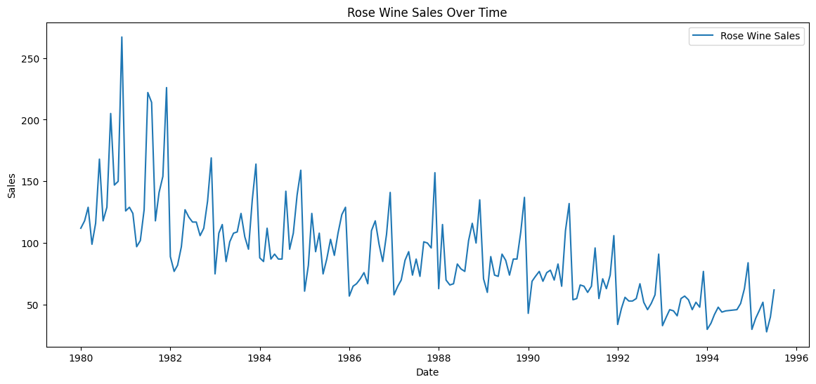
You can see clear seasonality with peaks recurring about every 12 months, and an overall downward trend.
Step 2: Selecting SARIMA Parameters with Auto-ARIMA
Choosing the right (p, d, q)(P, D, Q, m) parameters can be tricky when you start.
But pmdarima library’s auto_arima automates this by searching for the best combination based on information criteria like AIC.
print("Auto ARIMA and Auto SARIMA for Rose Wine")

# Auto ARIMA for Rose
auto_arima_rose = auto_arima(
    train_rose['Rose'],
    seasonal=False,
    trace=True,
    error_action='ignore',
    suppress_warnings=True,
    stepwise=True
)
print("Best Auto ARIMA Model for Rose Wine:")
print(auto_arima_rose.summary())

# Auto SARIMA for Rose
auto_sarima_rose = auto_arima(
    train_rose['Rose'],
    seasonal=True,
    m=12,
    trace=True,
    error_action='ignore',
    suppress_warnings=True,
    stepwise=True
)
print("Best Auto SARIMA Model for Rose Wine:")
print(auto_sarima_rose.summary())
What we get are estimated model parameters and diagnostics, helping us understand the model structure and fit quality.
                                      SARIMAX Results
============================================================================================
Dep. Variable:                                    y   No. Observations:                  149
Model:             SARIMAX(2, 1, 2)x(1, 0, [1], 12)   Log Likelihood                -663.811
Date:                              Sat, 16 Nov 2024   AIC                           1341.622
Time:                                      14:25:44   BIC                           1362.602
Sample:                                  01-01-1980   HQIC                          1350.146
                                       - 05-01-1992
Covariance Type:                                opg
==============================================================================
                 coef    std err          z      P>|z|      [0.025      0.975]
------------------------------------------------------------------------------
ar.L1         -0.4717      0.235     -2.006      0.045      -0.933      -0.011
ar.L2         -0.0623      0.102     -0.610      0.542      -0.263       0.138
ma.L1         -0.2522      0.236     -1.071      0.284      -0.714       0.209
ma.L2         -0.6059      0.238     -2.551      0.011      -1.071      -0.140
ar.S.L12       0.9854      0.017     58.956      0.000       0.953       1.018
ma.S.L12      -0.7863      0.118     -6.652      0.000      -1.018      -0.555
sigma2       402.8422     45.772      8.801      0.000     313.131     492.553
===================================================================================
Ljung-Box (L1) (Q):                   0.05   Jarque-Bera (JB):                77.80
Prob(Q):                              0.83   Prob(JB):                         0.00
Heteroskedasticity (H):               0.20   Skew:                             0.80
Prob(H) (two-sided):                  0.00   Kurtosis:                         6.17
===================================================================================
Step 3: Forecasting with Confidence Intervals
A lot of DS and ML projects are going to require you to try a ton of things and pick the winners, so tons of trial and error.
This is what I had for RMSE across different params:
| Model            | Order     | Seasonal Order   | RMSE       |
|------------------|-----------|------------------|------------|
| AR               | (2, 0, 0) | None             | 50.691553  |
| ARMA             | (2, 0, 2) | None             | 26.107300  |
| ARIMA            | (1, 1, 2) | None             | 20.889614  |
| SARIMA           | (1, 1, 2) | (0, 1, 1, 12)     | 11.258172  |
| Best Auto ARIMA  | (2, 1, 3) | None             | 19.700298  |
| Best Auto SARIMA | (2, 1, 2) | (1, 0, 1, 12)     | 10.474901  |
After fitting, forecasting is straightforward.
best_auto_sarima_model_full = SARIMAX(rose_data['Rose'], order=(2, 1, 2), seasonal_order=(1, 0, 1, 12)).fit(disp=False)

# 12 month forecast
forecast = best_auto_sarima_model_full.get_forecast(steps=12)
forecast_index = pd.date_range(rose_data.index[-1] + pd.DateOffset(months=1), periods=12, freq='M')
forecast_mean = forecast.predicted_mean

# 95% and 99% confidence intervals
forecast_conf_int_95 = forecast.conf_int(alpha=0.05)
forecast_conf_int_99 = forecast.conf_int(alpha=0.01)

forecast_mean.index = forecast_index
forecast_conf_int_95.index = forecast_index
forecast_conf_int_99.index = forecast_index

# Forecast table
forecast_table = pd.DataFrame({
    'Forecast': forecast_mean,
    'Lower 95%': forecast_conf_int_95.iloc[:, 0],
    'Upper 95%': forecast_conf_int_95.iloc[:, 1],
    'Lower 99%': forecast_conf_int_99.iloc[:, 0],
    'Upper 99%': forecast_conf_int_99.iloc[:, 1]
})

forecast_table.reset_index(inplace=True)
forecast_table.rename(columns={'index': 'Date'}, inplace=True)
print("12-Month Forecast with 95% and 99% Confidence Intervals for Rose Wine:")
print(forecast_table)
This is the actual forecast with the confidence intervals.
| Date       | Forecast   | Lower 95% | Upper 95% | Lower 99% | Upper 99% |
|------------|------------|-----------|-----------|-----------|-----------|
| 1995-08-31 | 43.32      | 7.38      | 79.27      | -3.92     | 90.57     |
| 1995-09-30 | 42.48      | 5.11      | 79.84      | -6.63     | 91.58     |
| 1995-10-31 | 45.28      | 7.88      | 82.67      | -3.87     | 94.43     |
| 1995-11-30 | 54.49      | 16.67     | 92.31      | 4.79      | 104.19    |
| 1995-12-31 | 81.95      | 44.02     | 119.88     | 32.10     | 131.80    |
| 1996-01-31 | 21.22      | -16.90    | 59.34      | -28.88    | 71.31     |
| 1996-02-29 | 29.91      | -8.37     | 68.19      | -20.40    | 80.22     |
| 1996-03-31 | 36.13      | -2.31     | 74.58      | -14.39    | 86.66     |
| 1996-04-30 | 36.91      | -1.70     | 75.53      | -13.83    | 87.66     |
| 1996-05-31 | 30.52      | -8.26     | 69.30      | -20.44    | 81.49     |
| 1996-06-30 | 36.76      | -2.18     | 75.70      | -14.42    | 87.94     |
| 1996-07-31 | 46.87      | 7.77      | 85.98      | -4.52     | 98.27     |
And the following code gives us our forecast chart with the confidence intervals.
plt.figure(figsize=(12, 6))
plt.plot(rose_data.index, rose_data['Rose'], label='Historical Sales', color='blue')
plt.plot(forecast_index, forecast_mean, label='12-Month Forecast (Auto SARIMA)', color='purple')

# 95% Confidence Interval
plt.fill_between(forecast_index, forecast_conf_int_95.iloc[:, 0], forecast_conf_int_95.iloc[:, 1],
                 color='purple', alpha=0.2, label='95% Confidence Interval')

# 99% Confidence Interval
plt.fill_between(forecast_index, forecast_conf_int_99.iloc[:, 0], forecast_conf_int_99.iloc[:, 1],
                 color='purple', alpha=0.1, label='99% Confidence Interval')

plt.title('12-Month Future Forecast for Rose Wine with 95% and 99% Confidence Intervals')
plt.xlabel('Date')
plt.ylabel('Sales')
plt.legend()
plt.show()
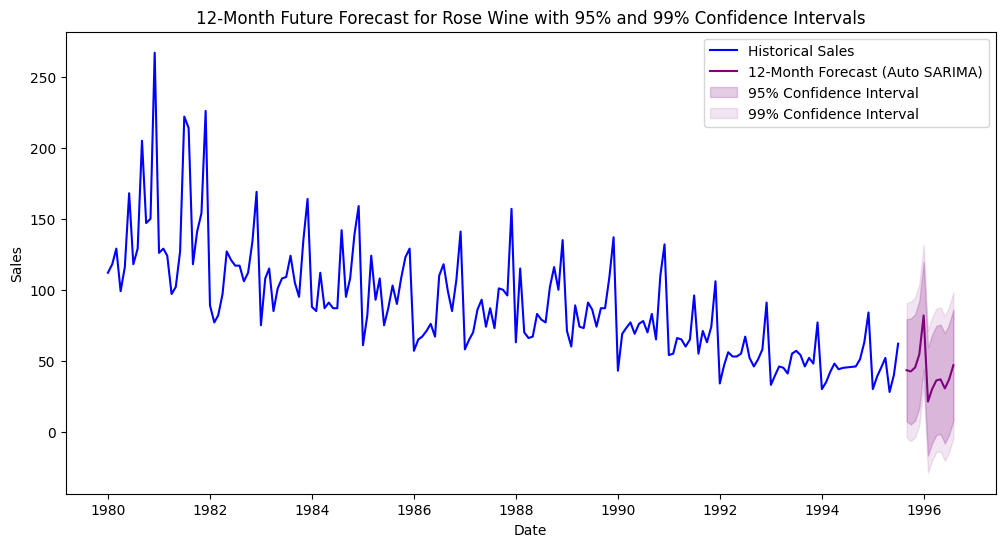
The confidence intervals are extremely important, they show the stakeholders how much inherent risk exists in these predictions. And of course this tends to be missing in a ton of black-box models.
Common Issues and Tips When Using ARIMA/SARIMA
- Misinterpreting Confidence Intervals: The intervals give us model uncertainty assuming the model is correct; they do not guarantee future observations will fall within them.
- Ignoring Differencing: Not differencing non-stationary data will give you poor model fit and unreliable forecasts.
- Mistaking Noise for Trend: Overfitting to noise can happen if parameters are too large; use information criteria and diagnostics to avoid this.
- Seasonality Mismatch: Seasonal period
mmust match your data frequency (e.g., 12 for monthly, 4 for quarterly). - Data Quality: Missing values or outliers will distort model estimation; preprocess like a pro please.
- Overreliance on Automation: Auto-ARIMA is helpful but understand the underlying assumptions and validate results.
Time Series Deserves a Comeback in the ML Toolkit
I’ll be honest - I love deep learning. It’s exciting, and super fun to play with. But when it comes to time series forecasting in real-world business scenarios?
It’s not always the best fit.
Most business data is small, seasonal, and needs to be explained to someone who doesn’t care about neural networks. That’s where ARIMA and SARIMA really help out.
They’re simple, fast, and surprisingly effective.
And they make it easy to say why something was forecasted the way it was.
Want to Dive Deeper?
If you want to build stronger intuition around time series forecasting, try applying ARIMA/SARIMA to your own datasets and experiment with parameter tuning and of course let me know how it goes!